1. Introduction and Problem Formulation
  2. Conventional solutions to the problem
  3. Self-Organizing Mapping (SOM)
  4. Dimensionality Reduction (KL Transformation)
  5. Experimental Results
  6. Conclusions
  Reference

1. Introduction and Problem Formulation

An important scientific activity is to collect the results of measurements. In the area of medicine, modern physical measuring methods provide an ever increasing amount of information. For example, clinical examination and complementary investigation, such as biochemical analyses, result in a large possible a picture of the physiological (normal or abnormal) status of a patient. Because of the availability of modern computer data-acquisition methods, the assembling and storing of data has become more and more necessary, and proper target-interpretation of these data has received more and more attention resulting in a better utilization of the available information.

Pattern recognition is a mathematical discipline that tries to extract and utilize information from a large amount of real or complex data. In pattern recognition, measurements on samples, objects, phenomena, etc. are used for a classification purpose on an objective and formal basis. In medicine, the purpose of pattern recognition is the fitting of patients into a well defined class [1].

Recall that comparison of many classification methods based on a set of thyroid gland data which consists of 5 laboratory tests relating to the thyroid function, has been done by Dr. Coomans in [2]. The data were collected for 215 patients divided in 3 classes, including euthyroidism (normal), hypothyroidism and hyperthyroidism. In that study 18 discrimination techniques were compared on the basis of correct classification rates, probability performance criteria and reliability. These techniques included k-nearest neighbor classification, linear learning machine, Bayesian classification on the basis of normal distributions and equal variance for the training classes, and many more. Some results have been observed from the comparison of correct classification rates for the different classifications. First, in the normal/hypo differentiation the probabilistic k-NN method performs less well than the non-probabilistic alternatives 1-NN and k-NN. Second, although the simple histogram method – Bayesian classification on the basis of frequency histograms is considered as primitive compared to the other techniques, it behaves very well in the study. Finally, the poor performance of some techniques may be due to the fact that in the normal/hypo differentiation some of the laboratory tests are redundant, which is not the case for the normal/hyper differentiation.

In this work, the thyroid gland functional data is used to test different pattern recognition methods. The thyroid data are collected from three classes. Let , , and  denote the class of normal thyroid function, hyper-thyroid function, and hyperthyroid function, respectively. An unknown pattern in each class is represented by a feature vector , where . First, conventional classifiers are applied to the data without dimensionality reduction, including Bayes method, Linear classifiers, and 1-NN. A kind of neural network, Kohonen Self-Organizing Mapping (SOM) [3, 4], is also used to the original data. Second, we use KL transformation to reduce the dimension of the sampled data, then input the transformed data to the four classifiers used previously, including the SOM neural network. In this problem, since some information is lost after KL transform, the misclassification rates increase in the low dimension case.

The remainder of this paper is organized as follows. In section 2, we overview some conventional methods to the classification problem. In section 3, the neural network - SOM is introduced to the problem. We discuss in detail the architecture of the SOM system, the procedure of SOM, and the method of selecting some critical parameters of SOM. The KL transformation method is presented in section 4. We give the numerical results of conventional methods and SOM in section 5. In section 6, we summarize the work and give our conclusions.

2. Conventional solutions to the problem

Some popular classifiers are considered in this section. Since it is a problem in the three-class case, we discuss below the multi-class version of each kind of classifier [5].

2.1 Bayes Classifier

Bayes decision theory is a fundamental statistical approach to the problem of pattern recognition. This approach is based on the assumption that the decision problem is posed in probabilistic terms, and that all the relevant probability values are known.

Let us focus on the three-class case. The first assumption of Bayes classifier is that the a priori probabilities , , and  are known. In practice, they can easily be estimated from the available training feature vectors. Let denote the total number of available training patterns, and , , and  of them belong to class , , and , respectively, then , , and . The other statistical quantities assumed to be known are the class-conditional probability density functions , describing the distribution of the feature vectors in each class. If we assume that  follow the general multivariate normal density, the problem of estimating  is reduced into that of estimating the mean value and the covariance matrix of the class, as we will discuss later. Recall that the Bayes rule can be described as

,

where  is the probable density function of . Then the Bayes classifier can now be stated as

If and ,  belong to ,

If and ,  belong to ,

If and ,  belong to .

For the thyroid gland data, a Bayes classifier is designed with assumption that all the data in each of the classes are generated from the normal distribution. Now, the class-conditional probability density functions of the class in the 5-dimensional feature space can be written as

,

where  is the mean of the  class and  denotes the 5-by-5 covariance matrix defined as

.

Let us define the discriminant functions, which involve the logarithmic function:

.

After removing the constant part of , we obtain the new discriminant function which represents a quadratic surface:

,

where

,

,

and

.

Bayes classifier can now be designed by using the discriminant function as:

If and ,  belong to ,

If and ,  belong to ,

If and ,  belong to .

2.2 Linear Classifier

Linear classifier is another kind of widely used classifier, since in some cases, the resulting classifiers are equivalent to a set of linear discriminant functions. For example, a Bayes classifier with assumption of equal covariance matrix for each of the classes. In this section, we will design the optimal linear classifiers by adopting some appropriate optimality criterions.

Let us consider the thyroid data in the three-class case. Then our task is to devise three decision hyper-planes in the 5-dimensional feature space, each of which can be given by:

,

where  is known as the weight vector and  as the threshold.

2.2.1 Fisher Criterion

It is well know that in the one-dimensional, two-class problem Fisher criterion for the linear classifier is the optimal one. But it doesn't work for more than two classes. Because we discuss the 3-class case, we extend the Fisher Criterion to the multi-class case. In fact, when the number of classes is larger than 2, the criterion is called the trace optimization procedure.

Let

,

,

where  denotes the number of classes,  and  are the covariance matrix and the mean value of the  class, and  is the mean of all the data. Then the criterion can be expressed as:

,

where A is a matrix. Let

,

.

Then we calculate the eigenvectors of  corresponding to the non-zero eigenvalues. Each eigenvector will be the column of A. After the procedures above, the dimensionality of the input data is reduced automatically down to the 2-dimensions for the 3 classes. We then keep only the first feature. Thus, all the data are projected into one dimension along the orientation of the left feature. By searching in this direction, we can obtain two thresholds to optimally classify three classes in one dimension.

2.2.2 Bayes method with assumption of equal covariance matrix for each class

As mentioned before, if we assume equal covariance matrices for each class, we also can design a linear classifier by the Bayes rule.

Similar to the Bayes classifier, let

,

and



where . The decision rule is the same as that of the Bayes classifier discussed previously.

2.3 1-NN Classifier (leave-one-out)

The k-NN density estimation technique belongs to the nonparametric method of pattern classification. Although it doesn't fall in the Bayesian framework, it results in a suboptimal in practice. The algorithm for the nearest neighbor can be summarized as follows. Given an unknown feature vector and a distance measure, then:

1. Out of the N training vectors, identify the k nearest neighbors, k is chosen to be odd.
2. Out of these k samples, identify the number of vectors, , that belong to class .
3. Assign  to the class with the maximum number  of samples.
Various distance measures can be used, such as the Euclidean and Mahalanobis distance. For the thyroid data, the simple version of this algorithm, 1-NN rule, is used, because of the limited sample data. In other words, a feature vector is assigned to the class of its nearest neighbor.

It is known that the classification error of the 1-NN with the resubstitution procedure is always zero. Because the nearest neighbor of a feature vector is always itself. So, we choose an alternative method of 1-NN, which is known as the leave-one-out method. This method alleviates the lack of independence between the training and test set in the resubstitution method. The training is performed using N-1 samples, and the test is carried out using the excluded sample. If this is misclassified an error is counted. This is repeated N times, each time excluding a different sample.

3. Self-Organizing Mapping (SOM)

Self-Organizing Mapping is a kind of neural network, the idea of which comes from the research of the functions of the human brains. The SOM algorithm was presented in 1985 by Dr. Kohonen. In his book [3], he states that a property which is commonplace in the brain but which has always been ignored in the learning machines is a meaningful order of their processing units. "Ordering " usually does not mean moving of units to new places. The units may even by structurally identical; the specialized role is determined by their internal parameters which are made to change in certain processes. It then appears as if specific units having a meaningful organization were produced.

Although a part of such ordering in the brain were determined genetically, it will be intriguing to learn that an almost optimal spatial order, in relation to signal statistics, can completely be determined in simple self-organizing processes under the control of received information. It seems that such a spatial order is necessary for an effective representation of information in the internal models. The various maps formed in self-organization are able to describe topological relations of input signals, using a one- or two-dimensional medium for representation. Such dimensionality-reducing mappings seem to be fundamental operations in the formation of abstractions.

From another point of view, the SOM algorithm belongs to the class of competitive learning schemes (CLS). These schemes employ a set of representatives . Their goal is to move each of them to regions of the vector space that are dense in vectors of the input data. It must be emphasized that competitive learning algorithm do not necessarily stem from the optimization of a cost function.

The general idea of the SOM algorithm is very simple. When a vector x is presented to the algorithm, all representatives compete with each other. The winner of this competition is the representatives  that lies closer to x according to some distance measure. Then the winner is updated so as to move toward x, while the losers either remain unchanged or are updated toward x but at a much slower rate.

3.1 SOM algorithm

To introduce the basic self-organizing process, we use the following array of the figure 3.1 for illustration.

 Figure 3.1: Two-dimensional self-organizing system Consider the thyroid gland data. Let each unit receive the same scalar signals , then the output of the representative j can be written as:  

,

where  are the adaptive weights. In fact, every ordered set may be regarded as a kind of image that shall be matched or compared against a corresponding ordered set ; our goal is to devise adaptive processes in which the parameters of all units converge to such values that every unit becomes specifically matched or sensitive to a particular domain of input signals in a regular order.   Instead of considering the maximum output response, the location of the maximum may also be regarded as defining the best match between the input vectors and the weight vectors . Widely applied matching criterion is the Euclidean distance between vectors. If we define the best match to be due at unit with index , then can be determined by the condition:  

.

For the processing units of the array, some model law of the basic adaptive units should be chosen. The adaptation equation may be of the form:  

      for   ,

where  denotes a topological neighborhood which is defined such that all units that lie within a certain radius from unit are included in  and  is the gain sequence, which is usually a slowly decreasing function of time.   Now the SOM algorithm can be summarized as follows.

• t=0
• Initialize the topological neighborhood and the gain sequence .
• Repeat

t = t +1

Present a new selected feature vector to the algorithm

Determine the winning representative , according to the matching criterion

Parameter Updating

  for ,

  otherwise

End

• Until convergence has occurred OR 
• Identify the clusters represented by  's, by assigning each vector  to the cluster that corresponds to the representative closest to .

A proper choice for and  can best be determined by experience. Certain "rules of thumb" can be invented easily after some experience. Moreover, it may be useful to notice that there are two phases in the formation of maps that have a slightly different nature, that is, initial formation of the correct order and final convergence of the map into asymptotic form. For good results, the latter phase may take 10 to 100 times as many steps as the former, whereby a low value of  is used.   Once again, we emphasize that many experiments have indicated the following general rules to form the basis of various self-organizing processes:

• Locate the best matching unit.
• Increase matching at this unit and its topological neighbors.

 
4. Dimensionality Reduction (KL Transformation)

The basic concept of dimensionality reduction is to transform a given set of measurements to a set of features. If the transform is suitably chosen, transform domain can exhibit high "information packing" properties compared with the output samples. This means that most of the classification-related information squeezed in a relatively small number of features, leading to a reducing necessary feature space dimension.

The KL transformation is a popular method of reducing dimensionality. Let denote the feature vector in the thyroid data. The goal of the KL transform is to generate features that are optimally uncorrelated. Let

 

,

and A is chose so that its columns are the orthonormal eigenvectors of the correlation matrix of the feature vectors. Furthermore, if we assume the positive definite, the eigenvalues are positive. The resulting transform is known as the KL transform and it achieves the original goal of generating mutually uncorrelated features.

5. Experimental Results   In this section, we show the performance of the conventional classifiers and SOM method. We also show the effect of the KL transform on the classification problem. The thyroid data are used for all these classifiers.   First, let us consider the conventional methods including Bayes, Linear classifier and 1-NN. The total 5 features of the thyroid data are retained. The classification errors of each method are listed in Table 5.1:  

Table 5.1: Comparison of four popular classifiers.
 

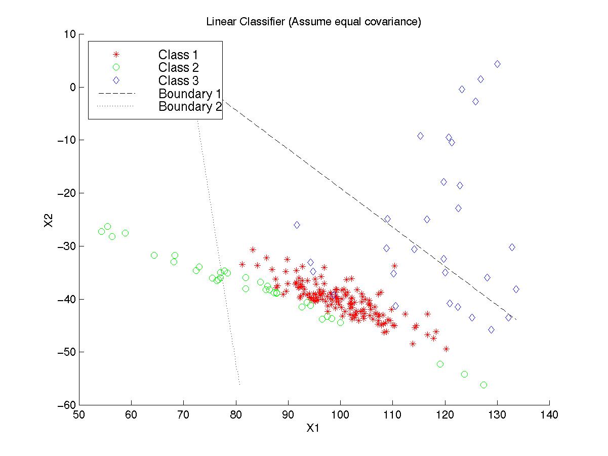
Note that Bayes classifier gives the best result, since the error rate of it is the lowest among the four classifiers. Also, we remark that Bayes classifier makes a resubstitution procedure, while 1-NN uses the leave-one-out method. So, we cannot say Bayes is better than 1-NN from the results above. Since the error rate of linear classifier is as high as 11.63%, the thyroid data are not linearly separated.   Then the KL transformation is applied to the thyroid data. We only keep the first two main features from the KL results. That is, the dimension of the data is reduced from 5 to 2. Mainly because we want to plot the boundaries of each classifier in the 2-D space. Table 5.2 shows the experiment results of the same four classifiers after KL transform.  

Table 5.2: Comparison of four classifiers after KL transform.
 

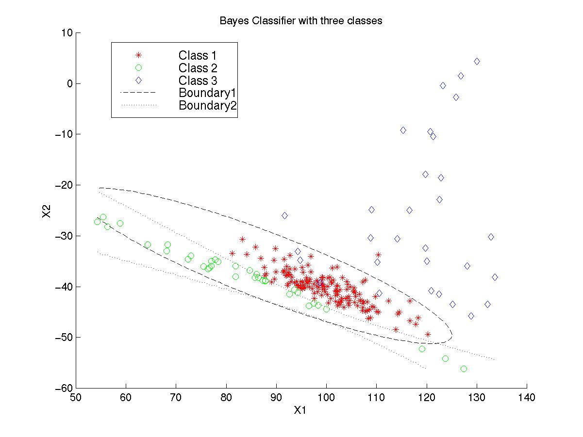
We note that Bayes again outperforms all other classifiers. But the error rates of each method are higher than those before KL transform. The reason is that some important features of the thyroid data are lost in the procedure of KL transform. As mentioned previously, after KL transform, we can show the decision boundaries of all the classifiers. We show the boundaries of linear classifier, Bayes and linear-Bayes methods in the 2-D case in the Figure 5.1, 5.2, and 5.3, respectively.  
Figure 5.1: Decision Boundaries of Linear Classifier. (Click here:  Figure 5.1 )

Figure 5.2: Decision Boundaries of Linear-Bayes Classifier. (Click here:  Figure 5.2 )

Figure 5.3: Decision Boundaries of Bayes Classifier. (Click here:  Figure 5.3 )
 

From these figures, we explicitly know how each conventional classifier works.   Now, let us consider the SOM neural network. We first take half of the data as the training data, and the remains as the testing data. Then we make a resubstitution test, that is, all the data are used to train the SOM, and then use them again to test the SOM. The gain sequence in the SOM is chosen as , and the maximum number of iteration is 10000. We give the results of such two tests in the Table 5.3.  

Table 5.3: The Error Rates of SOM.
 

Compare the results in Table 5.1, 5.2, and 5.3, we note that the performance of the SOM is not better than that of Bayes and 1-NN methods, it is only better than the linear classifier. The main reason is that the training data are not sufficient. In the thyroid database, there are only 35 vectors for the class of hyperthyroid function and 30 vectors for the hypothyroid function. Another reason is that the relative quantities of three classes data are not similar. 150 vectors are for the normal functional data, which is 5 times as many as the other two classes. To show how the SOM works explicitly, we give a map of the 2-D representations in the Figure below.  
We make the representations as a 7-by-7 array. Each square block denotes one output of the SOM system. After the training, we see that the data of each class cluster to a different region in the 2-D representations. When testing, if the data from one class is mapped into the corresponding regions in the 2-D space, then the classification of the data is right. Otherwise, it is an error. Also note that the 2-D representation after KL transform is a little bit intercrossed, because two blocks representing the class 2 are located in the region of the class 1. That is the reason why the error rate of KL-SOM is higher than that of SOM.

7. Appendix

We have the MATLAB codes for all the classifiers discussed above, including the Self-Organizing Mapping. If you have any questions about this report or if you are interested in our MATLAB codes, please feel free to contact us at:

kun@dsp.ufl.edu