Spectrum Sharing via Sequence Design - Supplementary Material |
|---|
Spectrum Sharing via Sequence Design - Supplementary Material |
|---|
This webpage contains the supplementary images from the (submitted for review) IEEE Signal Processing Magazine Tips and Tricks article "Spectrally Constrained Waveform Design". This webpage constains the SHAPE function (in MATLAB), examples (in MATLAB) and further discussion on the practical consideration for using the SHAPE algorithm. This page also contains more images regarding the examples presented in the paper as well as the MATLAB scripts used to generate all the images.
Errata: Equation 6 should be a minimization with respect to the x vector and not to z.
| Step by Step Guide to Implementing SHAPE | |
|---|---|
|
|
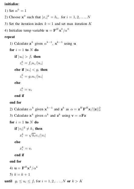
This is the SHAPE algorithm presented in a step by step format. We begin by initializing the alpha parameter and picking a sequence x that has a the required complex envelope. It is recommended to choose alpha to be 1 at this point, but that is not necessary. If alpha is chosen to be a complex number it will result in a constant phase offset being applied to the output. We then set the initialization counter k to be 1 and choose a max iteration amount. Typically 50000-100000 iterations is more than adequate.
Next we begin the SHAPE algorithm. We start by solving the first sub-problem minimize z with respect to (w.r.t) alpha and x. We use a temporary variable u to first evaluate the non-constrained minimizer. The vector u can be calculated via a scaler product and 1 FFT operation of x. Then we check the constraint and appropriately assign the magnitude and phase to the new spectrum vector z. There is no dependency between any iteration of the for loop and this could be implemented very quickly using parallel processing
The next step is to solve the unconstrained minimization of alpha w.r.t z and x. This is an inner product and 1 scalar division operation.
The last step per iteration is to minimize x w.r.t. z and alpha. Again we use a temporary variable v which can be calculated using the IFFT operation on z and a scalar-vector product. The optimal x use the phase of v, but has the required envelope. Again the for loop is independent of all other iterations and could be implemented using parallel processing.
We then check to see if the vector changed. Note that if u was within the bounds then z is equal to the FFT of x. Then alpha would be equal to 1. Hence the new x calculated in this iteration would be the same as before and the cost function would be zero. The algorithm will also end if some max iteration threshold has been met.
| Guard Bands for Better Convergence | |||
|---|---|---|---|
|
|
||
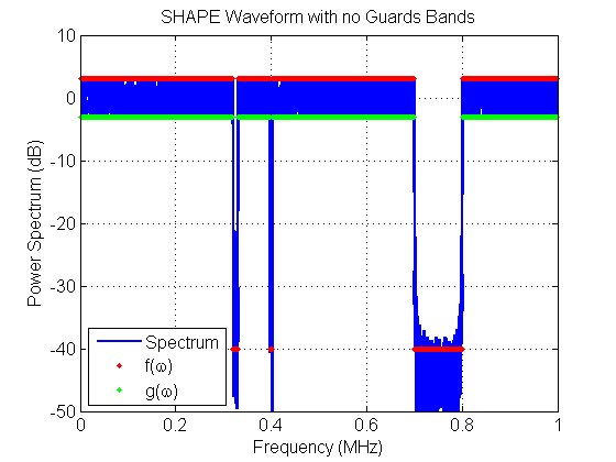
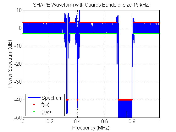
There is no guarantee that the SHAPE algorithm will converge for a given time domain complex envelope and a set of bounds. To help promote the convergence of the SHAPE algorithm we suggest including guard bands near steep spectral transitions. These guard bands can be small spectral regions near the transition regions.
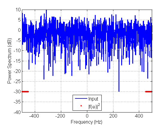
We demonstrate the problem and the resolution using a simple example. Consider designing a notched random phase sequence with bandwidth 1 MHz and unimodular complex envelope. The power spectrum shape allows +/- 3 dB ripple in the passband and that stopband notches to be -40 dB down with widths of 10, 1 and 100 kHz. The left hand figure above shows the power spectrum of the SHAPE waveform when using the strict limits. The red line corresponds to the upper bound and the green line corresponds to the lower bound. After 60000 iterations SHAPE was terminated and examination of the cost function shows it was oscillating around a non-zero value. This is most likely due to the sharp transitions in the spectrum shape introducing a large amount of ringing which was conflicting with the spectral bounds.
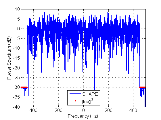
To overcome this we introduce 15 kHz guard bands on both sides of each spectral notch. The right hand figure above shows the SHAPE output when initialized with the same unimodular random phase sequence as the left hand side. When the spectrum constraints were relaxed, SHAPE was able to converge to a zero cost value within the 60000 iterations. We see that by allowing some freedom in the passband the deep notches can be achieved at the cost of a degraded passband, which should be acceptable in many practical applications.
We have included the script used to generate the above plots. It should be noted that the -40 dB notch is quite difficult and SHAPE may not converge even with the 15 kHz guard bands. However, it can converge as shown in the above plots. Reducing the notch width to -30 dB greatly increases the probability that SHAPE converges.
| Quantization Effects | |||
|---|---|---|---|
|
|
||
|
|
||
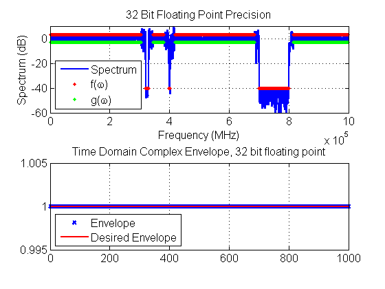
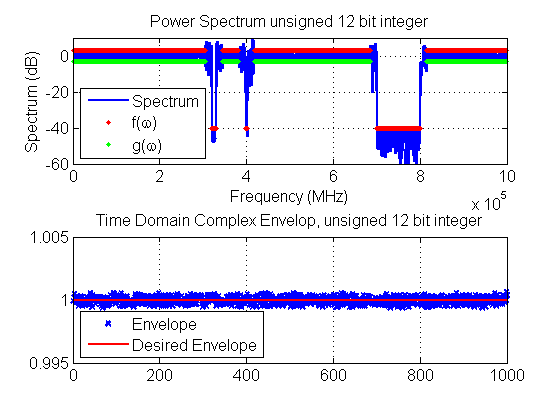
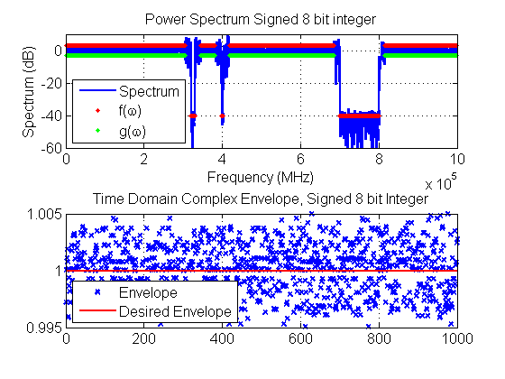
In this section we examine the effects of using finite precision on the SHAPE waveforms. The SHAPE MATLAB fucntion uses a 64 bit floating point complex number representation which provides adequate numerical precision. In most realizable systems thought the arbitrary waveform generator will use typically a fixed point representation of the number with smaller bit precision. The provided script "Bit_Truncation.m" examines how the complex envelope and spectrum degrades as the precision decreases. The data provided in "EXAMPLE_SHAPE_DATA.mat" is the same data used for the plots shown in the Guard Band Example section above.
There does not seem to be a simple metric to describe exactly how the performance degrades due to loss of precision with SHAPE waveforms. However, from our empirical results 12-16 bits seems to be adequate for representing SHAPE waveforms. Test data from actual arbitrary waveform generators is currently being developed and will be added to this website when it is available.
| Initialization | |||
|---|---|---|---|
|
|
||
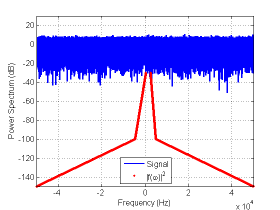
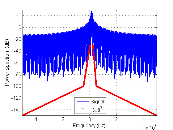
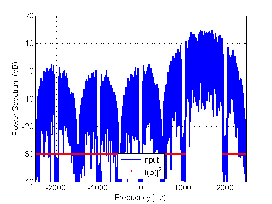
The initialization waveform used in SHAPE is very important. For example, if a system designer wishes to utilize a unimodular random phase sequence for an application that requires a passband of 1 kHz, but it will be oversampled at 100 kHz. We then want to use SHAPE to find a random phase waveform that meets steep spectral roll-off restrictions. One possible option for the initialization of SHAPE is to use a random phase waveform sampled at the maximum bandwidth 100 kHz. Another option is to use a sequence that is sampled at 1 kHz and then upsampled to 100 kHz. The upsampling technique used is a sample and hold method. If x(n) is our original sequence of length N and we upsample by M, then our upsampled waveform x2=((n-1)M+m) = x(n) for n = 1,2,...,N and m = 1,2,..., M.
The left hand plot above shows the first option which is a 100 kHz bandwidth randomphase signal. Here the red line corresponds to the strict spectral requirements. Using the 100 kHz bandwidth random phase signal as an input of SHAPE may result in slow convergence since the initial waveform and the requirements are so different. However, if we use the upsampled 1 kHz waveform as shown in the right hand figure, then SHAPE may have a better chance at finding a suitable waveform. Using this upsampling type approach is the basis of the tiered SHAPE waveform design that is discussed and illustrated in our final example.
| Wideband Radar Example Images | |||
|---|---|---|---|
|
|
||
|
|
||
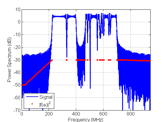
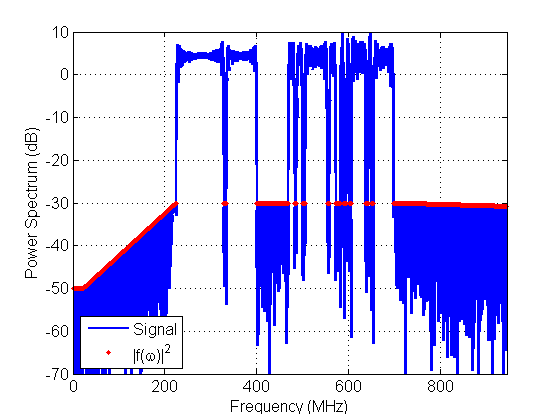
For the unimodular wideband radar example we have to generate a notched spectrum that avoids the unusable portions of the spectrum. The bands we must correspond to the following frequency bands (MHz): (328.6-335), (400.15-470), (482-486), (500-506), (554-560), (572-578), (590-596), (602-608), (638-644), (650-656), (674-680), and (680-686). We initialize SHAPE with the simple gapped LFM waveform seen above. The SHAPE waveform deepens the notches and significantly reduces the energy in the unwanted bands. It also has the sidelobes spectrally shaped to meet the National Telecommunications & Information Agencies spectral roll off requirements for a Group C radar. The sidelobes on the SHAPE waveform have increased, but they have not increased unreasonably. The performance is similar to the initial LFM waveform.
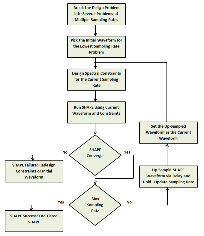
| Tiered SHAPE |
|---|
|
|
| Random Phase Sonar Example |
|---|
|
|
||
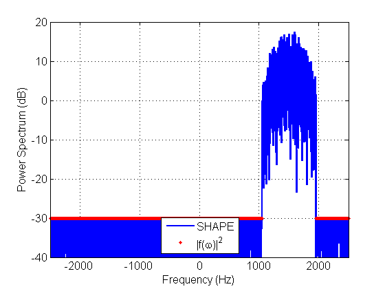
For Stage 1 we start with a random phase seqeune sampled at 1 kHz and limit the passband to 900 Hz. We can see in the SHAPE waveform output that the 50 Hz edges are suppressed 30 dB.
|
|
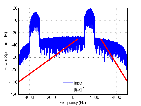
For stage 2, we take the stage 1 output and upsample it by a factor of 5 using a sample and hold approach. We then modulate the signal up to the desired carrier frequency of 1500 Hz. The upsampled and digitally shifted signal is our initialzer for the stage 2 SHAPE waveform. We must achieve -100 dB suppression by (+/-) 5000 Hz but we will do this step in stage 3. Instead we remove the sidelobes introduced via the upsampling method with SHAPE.
|
|
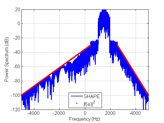
The stage 2 output is upsampled by a factor of 2 giving us a sampling rate of 10 kHz for stage 3. We will now utilize a linear ramp -30 dB to -100 dB. We also utilize guard bands of 500 Hz to allow for ripples and transitions as discussed in the section regarding convergence of the cost function to zero. The resulting mask occurs at frequencies 2500-5000 Hz and -5000 to 650 Hz.
|
|
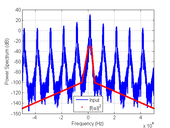
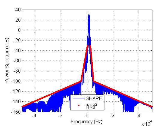
Stage 4 is the final stage and it upsamples the stage 3 output by a factor of 10. This results in the final sampling frequency of 100 kHz and we can set the complete spectral requirements. At the (+/-) 5000 Hz mark the spectrum must roll off at a lower rate but decreases to -150 dB by (+/-) 50000 kHz. The initial waveform shows the periodic repitition and spectral skirt due to the sample and hold approach to upsampling. SHAPE is able to suppress these unwanted repititions and find a sequence with the desired spectrum.
|
|
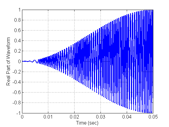
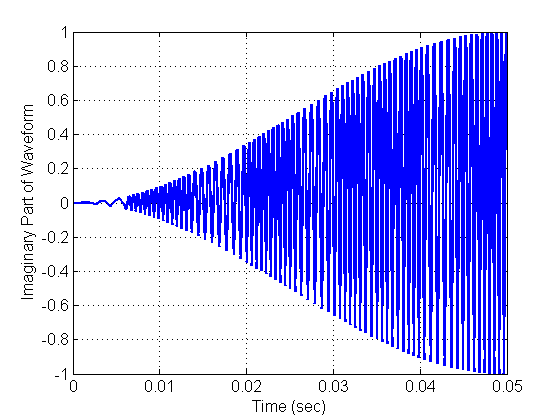
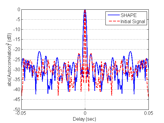
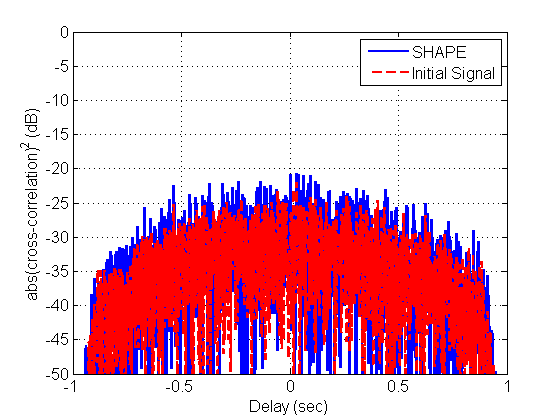
In this problem we have a Tukey window (with window parameter of 0.1) for our complex envelope shape. The pulse has a duration of 1 second so the rise and fall time accounts for approximately 10% of the pulse duration. We can also see that this is not similar to a linear frequency modulated waveform since the frequency seems to change in bursts and not in a linear manner.
|
|
||
|
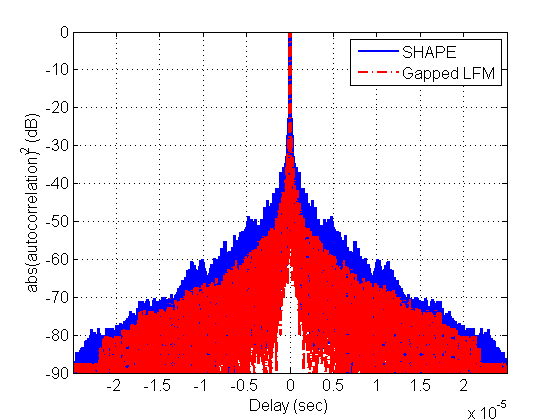
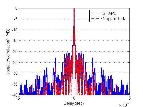
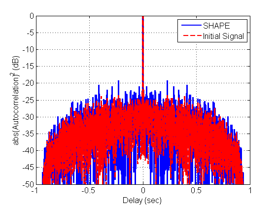
The autocorrelation of the output waveform and the input waveform (1000 Hz sampled random phase waveform). We see that the sidelobe levels are slightly higher for the SHAPE waveform, but they do not increase to much compared to the original random phase seqeunce. The mainlobe also widens which is expected due to the non-flat passband shape of the output waveform. We also generated a second sequence using a different random phase sequence. The cross-correlations (normalized to the max of the autocorrelations) show that the SHAPE waveform outputs are just as uncorrelated as the input random phase waveforms. This shows that SHAPE found 2 different sequences that met the spectral restrictions.